A “measure” of “complexity”

ALL WHICH IS WRITTEN HERE IS CRAP!
FOR A SLIGHTLY LESS CRAPPY DESCRIPTION
OF THIS “MEASURE” READ THIS:
https://thegrandmotherblogg.wordpress.com/wp-content/uploads/2014/05/document.pdf

 

In this post I will introduce a little method I figured out in order to “measure complexity”. I know that this method is most likely nothing new or useful by any stretch of the imagination but i had a lot of fun playing with it and trying to make it work. I came up with this method after having written a cellular automaton. The problem was that there where 2^64 different rules and some of them produced really cool and complex patterns but most where just random and boring. So i set out on the futile quest to find a way to identify these cool patterns automatically. The fact that the patterns i was trying to find was the patterns that made me go “ouu that is awesome!”  when I looked at them did not really aid in finding an algorithm to find them. So essentially I was trying to find a needle in a haystack when I had no real idea of what a needle was.

This project has been an epic one filled with elation and despair (mostly despair). Although i have been aware that the measure was “decent” ever since i first tested it i have run in to so many roadblocks and i have been so wrong so many times during this project that i frequently thought about just giving up, banishing this project to the crowded folder of failed ideas.

I will not publish any code used in this post due to it being so ugly that if you where to wake up next to it after a night of heavy drinking you would spend the day crying in the shower, vowing never again to drink alcohol. But if anyone of you desperately want the code just message me and i might consider it.

Overview

With no reason what so ever i thought that the best way to start where to try to find a good measure of the “complexity ” and that one way of doing that was with the following assumption/guess:

The complexity of a string is in some weird way proportional to the number of unique symbols in the run-length encoding of the string.

Okay so what do i mean by this:
Lets pretend that we have the following string 10110001101. The run-length encoding of that string would then be (1,1) (1,0) (2,1) (3,0) (2,1) (1,0) (1,1) where (a,b) is to be read as a number of b‘s. Then we consider how many unique (a,b) tuples there are. In this case there are 4 of these. Namely : (1,1) (1,0) (2,1) (3,0). So the string 10110001101 have a complexity of 4 in my measure. One interesting to view this is is that the string 10110001101 can be expressed in a language with a alphabet consisting of only (1,1) (1,0) (2,1) (3,0). This method can obviously be generalized to strings consisting of arbitrary many symbols.

I have also done some extensive but utterly failed attempts at some theoretical explanation for using this method as a measure of complexity. I have tried several different approaches but they have all been futile. Maybe i will give it a go after having taken a course in automaton theory.

The actual implementation of this method is very straight forward but for patterns which are constructed of several strings it becomes more difficult since one has to find a way to interpret the combined. How this was to be done was not obvious but after some extensive guessing i found some methods which worked.

Application

So maybe we would like to actually try to use this method to try to find something interesting about some automatons. So lets start with the elementary automaton which we all area familiar with. So lets just go out on a limb here and say that we want to compare the patterns generated by the different elementary cellular automatons using my measure of complexity in a vain attempt to be able to identify interesting behavior of the underlying set of rules. The problem which we are faced with now is determining how to use the measure in order to compare the different patterns.

Elementary CA

In all of these examples i will use patterns that are of the size 100*100 cells with an initial random configuration. The initial configuration will not be considered when we do the actual comparison. Each comparison is performed 50 times and then averaged. I will only compare the 88 different unique rules.

Don’t care about the actual values of the complexity score. We are only interested in comparisons between different patterns at this time.

Randall Munroe once wrote “i could never love someone who does not label their graphs” well… i say “i could never love someone who could not infer information from a context”.

Rule 110 is highlighted in the plots due to it being capable of universal computation and thus embodying the essence of a “cool” pattern.

Even though only the top 20 patterns are showed each method puts the lame(class one behavior ) patterns at the bottom of the list.

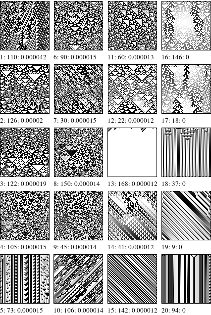
Total Complexity Method

Lets start with a pretty direct approach where we just add the complexity of both the rows and the columns of the pattern. We then end up whit this list:

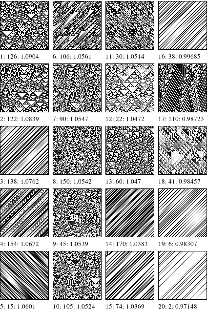
legend.
rank : rule : complexity

We can see that It picks out some interesting patterns for the top but otherwise there are a lot of bland and boring patterns in the top 20. The reason for this is that a pattern where all the lines/columns are very similar but have high complexity values will contribute to a higher overall value for the pattern.

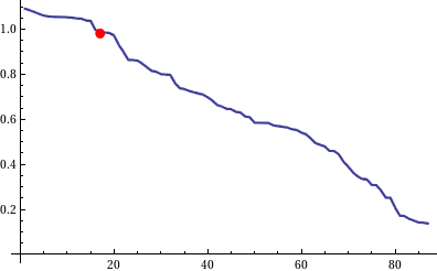
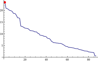
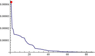
A plot of the sorted values of the complexity measures.
The red dot is rule 110

Looking at a plot of the sorted measures shows us another thing. Even though it might appear nice that the values seems to be distributed in a nice linear fashion we have no clear distinction between “cool” and “uncool patterns”.

Maximum Complexity Method

In a vain attempt to avoid the pitfalls of the above method lets sum up the maximum value of the complexity of the rows and the columns. And then we get:

legend.
rank : rule : complexity

We can see a slight improvement in the top patterns but there are still many boring patterns in the top 20. the same problem with just taking the total still appears here. So we are not there yet.

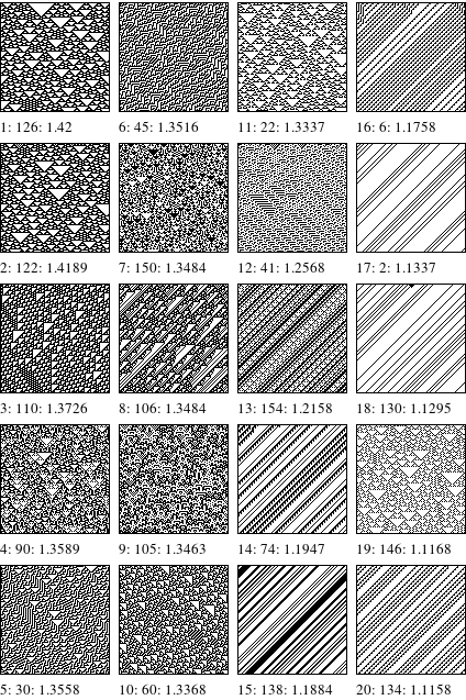
Recursive Method

Well in in a desperate attempt to avoid boring patterns where the individual lines / rows have great complexity making the way to the top. Lets try to avoid this by incorporating the complexity of the list of the complexity of each row /column to avoid patterns that have a repetitive nature. We do this as follows: Take the complexity of the string of complexity values and multiply it by the maximum value in the list of complexity values. Did anyone follow that? No probably not. But lets see what happens.

legend.
rank : rule : complexity

Well no we start to see some nice result. Lets just note that it picks Rule 110 as the coolest rule. Which is awesome but lets be a bit skeptical still since it could just be a onetime thing and just consider the fact that it seems to group all of the interesting patterns in the top.

Another nice feature is that it seems like the lamer patterns are all also somewhat grouped together by coolness.

Plot of the sorted complexity measures.
The red dot shows rule 110

Well this is nice. With some vivid imagination we can see distinct jumps which seem to correlate between the coolness of the patterns.

Variance Method

Another approached that can be used in order not to have repetitive patterns getting a high score is to make use of the the variance in of the complexity of the different rows and that of the different columns. This method works in an even weirder way than the previous one and don’t ask me how i came up with it since i just guessed. We get the measure M as follows:

Where Horizontal and vertical corresponds to the lists of horizontal and vertical values for the complexities.

Here we can see the results of using this method:

Legend
rank : rule : score

This method also picks out rule 110 as the top rule but then its appears to look a little bit worse since it tends to mix patterns of different “coolness” i.e rule 13 coming in at place 13 even though its a very boring rule.

Plot of the sorted complexity measures.
The red dot shows rule 110

We can see here on this plot that the second best rule is only half as good as the best one. One question now becomes weather or not this is a good or a bad thing. Its very hard to tell in this case since the dataset is so tiny.

Look-Back/Second-Order CA

Well as of now we have seen that this method is not useless and we have some support for believing that its not complete and utter crap. But lets put it to another test! We will now apply both the Variance Method and the Recursive Method to the Look-Back Cellular Automaton.

In these simulations i have used 5362 different rules for each of the methods tested. I have then plotted the sorted values of the measures obtained trough the two methods. I have also normalized the values of the measures for a clearer comparison.

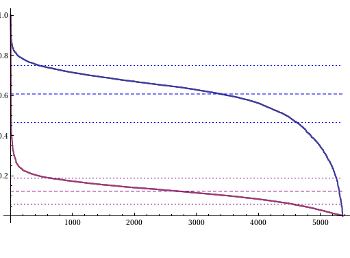
The Blu line is the distribution of the rules evaluated with the Recursive method and the Red is that of the rules evaluated with the Variance Method. The dashed line is the mean and the dotted line is the mean +- the standard deviation.

As we can see the Recursive method is way better distributed. Although on closer inspection we find that both methods have the same percentage of rules which has a score above one standard deviation from the mean. From the previous examples with elementary automatons we saw that both methods cases similar results to the same rules for the most cases. This indicates the usage of the Variance Method might be preferred since its way faster than the Recursion Method.

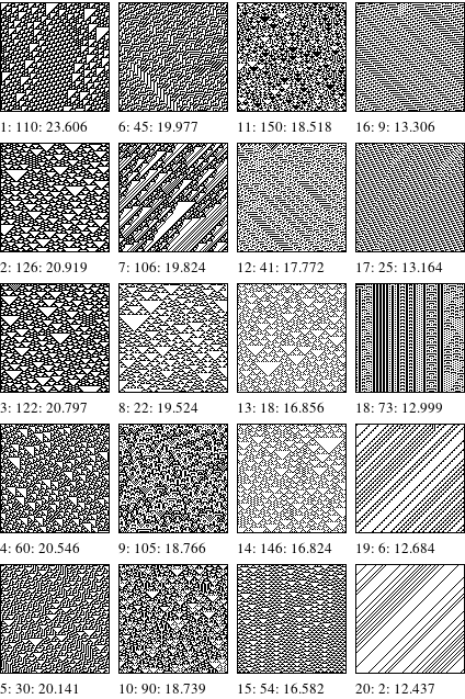
So lets see a few examples of some of the better rules generated by each method from the previous test.

#1 Variance Method

#2 Variance Method

#3 Variance Method

#10 Variance Method

#50 Variance Method

#100 Variance Method

#500 Variance Method

Well here we have a somewhat disappointing selection of some of the rules generated by the Variance Method. As we can see some really lame rules have jumped up to the top If one continues to search trough the top ranking rules one finds many many lame rules. Why this is i have no idea but its clear that the variance method is not as good which is a pain since its way faster than the Recurrence method. The loss of speed in the Recursion method might just be a problem of my implementation of the method for getting the complexity of strings of an arbitrary number of symbols.

So lets see weather or not the recursive method can perform any better.

#1 Recursive Method

#2 Recursive Method

#3 Recursion Method

#10 Recursive Method

#50 Recursion Method

#100 Recursive Method

#500 Recursive Method

Well well now it looks like something didn’t go totally wrong. Even tough the #1 pattern might look quite lame but if one shays hmm… scratches ones complete lack of a beard and look at it for a moment one will see that there is a actually a underlying structure so its not completely pointless. We can also see that all the others except number 500 are really really nice. Well all in all it looks like my method actually manages to find somewhat funny rules in the space of the rules for a second order cellular automaton.

Details

Don’t trust anything you see here. Its mostly crap.

Now it would be really nice to somehow normalize our measure. So that we can compare the complexity of two strings of unequal length. Why this is interesting is really not obvious since one might find it obvious that a longer string can have a greater complexity than a shorter one. It turns out that when we view complexity in this fashion the relationship between length and maximum complexity is not so obvious.

We must start by finding a way to construct the string having the highest complexity by our measure. To construct this string turns out to be very easily actually. we do this by simply following the easy pattern:1011001110001111000011111… this has the RLE: (1,1)(1,0)(2,1)(2,0)(3,1)(3,0)(4,1)(4,0)(5,1)… it is quite easy to see how this method generates the string with the highest complexity. So lets now ask another question: How long is the shortest string that have a complexity of 10 in our measure. The answer to this question is 30. Lets take a moment to consider why that is…
Lets just construct that string by taking the 10 shortest possible symbols in a RLE. That in this case being: (1,1)(1,0)(2,1)(2,0)(3,1)(3,0)(4,1)(4,0)(5,1)(5,0) and this then gives us the string: 101100111000111100001111100000 which is 30 characters long.This is not the only string of length 30 with a complexity of 10 but there is no string of length 30 with a complexity greater than 10.
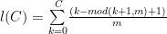
If one writes down some more examples and then stare at them in silent contemplation for a while one finds that the minimum length of a string having a maximum complexity of C is given by the formula:

Where m is the number of different letters in the string.

One neat thing to observer is that if we want to have a maximum complexity of 100 we would need a a string of length 2550 but to have a maximum complexity of 101 we would need to have a length 2601. So how do we solve the issue of finding the maximum complexity of a string of a given length. It turns out that there is a answer on a closed form if there string only contains two different symbols.

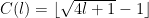
But for the case of a string consisting of more than two letters one can analytically find a interval in which C is for any given l and then its just a matter of brute forcing although finding a function for C given both a length and a arbitrary number of letters seems to be very non trivial.

One major thing which i have as of yet not been able to solve satisfactory is the mean complexity of a random string. This is a very important function which would enable some nicer comparisons than one can do without a good measure for it. Although some guessing and general button mashing gives us an approximation for large lengths as roughly:

Conclusion

Oh my God I’m so flippin tired of writing this post. I told myself that i should stop writing such long posts and here i sit with 2500 words of pure mediocreness. I doubt that anyone have bothered reading trough this entire text. I’m not even sure that i would.

But enough with the self pity. Al in all this project has been a great personal successes. I have actually had an idea that kinda works. There is a lot of work that can still be done but weather or not i ever get around to that depends on the response i get here.
I have learned a lot about how to structure a larger project and most of all the importance of proper and continuous testing.

Peace brothers!

Look Back Examples

This gallery contains 22 photos.

I’m sorry that wordpress rescales images like as if they where hamsters. These are some of the interesting rules which i have found for the look back automaton. All of these rules are for a nearest neighbor and one step look back rules. You can find a proper description of the automaton here.

The Look Back Automata

A “new” take on the cellular automaton

Introduction

In this post ill give a short introduction to a new little cellular automaton i made up. I am fully aware that this is most likely nothing new at all (EDIT: I have been informed that this type of automaton is what is called a second order automaton). But i have had a lot of fun developing the model, implementing it and studying the results. This model which i call a look back automaton is a variation of a simple one dimensional cellular automaton. I have found some of the patterns that i observed to be very fascinating a lot of them exhibit very intricate patterns and in a some of them its easy to identify specific parts corresponding to certain reactions and in some others i have observed one rule that spontaneously gave rise to the pattern you get from binary addition. But most importantly some of the  rules generate truly beautiful patterns that one could easily sell as art to some really stupid person with no taste at all.

The Java program can be found here

Overview

This model differs from the traditional one dimensional CA (from here on we will abbreviate cellular automaton by CA) in one key aspect. As the next state of a cell in a traditional CA depends only on the cells current state and that of it neighbors. But in the look back the new state of the cell depends on the current configuration of the neighborhood and the configuration of the neighborhood in the previous step/steps.

Nothing is stated regarding the size of the neighbor hood or how many steps in to the past one looks or even weather or not any previous  states are “skipped”. Although from here on i will only study the the case for a nearest neighbor (r  = 1) and a look back length of one. The number of possible rules  as to be expected are 2^(2^r*l) so for the case of the most trivial look back automaton the number of rules are 2^64 which is significantly larger than the 256 types of elementary CA that exists.

As you will see later on in the examples section most of the rules generated by the look back automaton are similar in behavior to those generated by  your standard one dimensional CA although some of the patterns differ greatly construction and appearance.

Implementation

I have written an implementation of this automaton in Java using a very straightforward approach. Since there exists only a finite number of different configurations of the neighborhood and thus only a finite number of transformation rules for each configuration is possible.  The easiest and most straight forward one of these is the case where there exists only two states for each cell. The rule can then be represented by a binary number that corresponds to a unique lookup table in a fairly trivial way.This is easily expandable for as system of arbitrary configurations but the implementation will be somewhat trickier.

I have chosen to let the field that hold the cells to be cyclic. The system then just needs to be given a startup configuration for the field and then one just applies the transformation rules for each cell in the last row of the field to obtain the configuration of the next row.

Examples

This is just very esthetically pleasing and also quite intricate.

This rule shows several different interesting patterns.

This rule spontaneously give rise to a pattern corresponding to addition.

You can find more examples here.

Further development

Since there exists a 2^64 number of rules for the most trivial look back configuration it would be very nice to have some reliable algorithm to search trough these rules with some algorithm that can in a somewhat reliable classify the different rules according to awesomeness. I have actually made some progress devising such a algorithm but i still have some work left to do and i think that if the algorithm turns out be useful it might warrant an dedicated post.

Ernst-Hugo Automaton Assembler

Ernst-Hugo Järegård being awesome.

I have been spending the entire weekend writing a assembler in Java for my automaton. I felt that i needed to give it a name while i worked on it so i have decided to call it the Ernst-Hugo Automaton after the Swedish actor and awesome person Ernst-Hugo Järegård. I  have used the the Automaton package that i wrote earlier with some changes. I had to change some of the scoping of the classes to make them work with the new Assembler package.

The code

The Assembler class is the a very ugly class which contains a constructor which acts as a main loop where the basic input parsing occurs. Most of the methods in the assembler class handles the parsing of the input but it also handles what is to be sent to be assembled and the running of the program. Valid assembly code is then sent from the Assembler class to the Program class when the assemble method in Program is called. The Program class is the program that you are working on. It contains both the assembly code for the program and the assembled program(given that it has been assembled). The Program class also contains the assemble method and the other methods needed for the assembling of the program. I know i should put this in a separate class… but i didn’t.

I have tried to write good looking code but i know that especially the Assembler class is mighty ugly. i  have also tried to implement some form of exception handling. There is also a somewhat extensive documentation of the classes used. I know that the documentation is rather incoherent and does not really adhere to any specific formating convention but i guess its better than nothing.

As of now the assembler does not implement that many features apart from some very basic editing of the input. It would be very nice to add things such as the ability to load and save programs. Right now the assembler cant handle any functions except for a function to add Jump lines.

The Automaton class contains some rudimentary unit testing methods. I really only wrote those for educational purposes and they can be pretty much disregarded but they are included just for fun.

The documentation can be found here.

The JAR containing the actual program and the source code can be found here. To run the program you will need to have a ANSI compatible command line interface or the program will look really stupid. It would not be that difficult to re factor it to normal output not using ANSI formatting. Just rewrite the AnsiDrawer class. It shouldn’t be that hard.

Operation

The operation of the assembler is pretty basic. The code is simply inputed using the symbols :
( 0 , 1 , . , ! , + , x , & , < , > ).  Which are the same as specified in previous posts although the symbols have been changed to ASCI equivalents.. The index (row) where the code will be added is shown before the “:” on each line. The index can be set by the commands which will be specified in detail later.

The jump command is implemented in this assembler and is typed as “#jump:pos:target”. Only one Jump will be added on a line and the rest of the line will be padded with Drop. You can add a Jump command with the target lying outside of the program. But when you assemble the program all Jump operators has to point to a line in the assembly code. Remember that all of the jump targets are absolute! so inserting lines in your program can screw up your Jumps.

The commands

All of the commands are preceded with a “§” symbol and are as follows:

new
Prompts the user for the memory size of the program and then creates a new Program instance. This has to be done before any code can be written. Calling new again will over ride any code or assembled program.

run
Runs the program given that it has been assembled. Prompts the user for a starting configuration of the memory. The program will run for a maximum of 200 steps in order to avoid infinite loops.

print
Prints out the assembly code.

assemble
Assembles the program. Will fail if any Jump targets lies outside of the program length. Prints the assembled code when done.

clear
Clears the screen.

help
Prints a help text.

set n
Will set the index to n. The index will then increment from n when a line of code is entered. All lines after n will be pushed down. Using set will screw up your Jumps if you are not careful.

replace n
Replaces line n with the next line of code entered. The index then returns to the end of the assembly code.

reset
Resets the index to the end of the assembly code

quit
quits the program.

Example

Here follows a little usage example. It is the 1 bit adder that i showed in the first post about this automaton. This example should give you a little better understanding of how the assembler works.

 0:§new
 Enter the memory size of the program:
 5
 You may now begin coding!
 0:.....
 1:.<.>.
 2:<>..x
 3:...<.
 4:.<>..
 5:.&<>.
 6:...&x
 7:..>..
 8:...+.
 9:§print
 0: .....
 1: .<.>.
 2: <>..x
 3: ...<.
 4: .<>..
 5: .&<>.
 6: ...&x
 7: ..>..
 8: ...+.
 9:§compile
 The command is silly! Use a propper one!
 9:§assemble
 Compiling: default
 0: DROP DROP DROP DROP DROP
 1: DROP CLONE_RIGHT DROP CLONE_LEFT DROP
 2: CLONE_RIGHT CLONE_LEFT DROP DROP XOR
 3: DROP DROP DROP CLONE_RIGHT DROP
 4: DROP CLONE_RIGHT CLONE_LEFT DROP DROP
 5: DROP AND CLONE_RIGHT CLONE_LEFT DROP
 6: DROP DROP DROP AND XOR
 7: DROP DROP CLONE_LEFT DROP DROP
 8: DROP DROP DROP OR DROP
 It would appear as if the program has compiled without any major trouble!
 9:§run
 Please enter the starting configuration
 00101
 00101
 0 00101
 1 00101
 2 01111
 3 10110
 4 10100
 5 11000
 6 11000
 7 11000
 8 11100
 G 11110
 Done!
 9:

Further development

I have been thinking a bit about writing some form of language for the system capable of some more complicated operations. I have figured out a way of creating a addressable memory space with the Ernst-Hugo automaton which would enable more advanced programming using a fixed but arbitrary word length. Although creating a new language would require a lot of  effort to implement but it would be really fun to be able to write more complicated programs for it. But that depends on the interest from you folks. If you really want me to write one i would definitely do it or if anyone of you would like to do that you are more than welcome! Just email me if you have any questions about the code or want to start a collaborative project with the Ernst-Hugo Automaton!

A simple automaton

A few days ago i had an idea for a simple automaton that could be used as a model of computation whose operation would be somewhat intuitive, powerful (Although not right now) and yet different from conventional models of computation to make it interesting. I am of course completely aware that this model probably is nothing more than a restatement of some other automaton. Although i would like to point out that i figured all of this out on my own though without any major interference from the real world. All of the coding has been done from scratch in Mathematica.

I will in this post give a very informal description of how the automaton works and i hope that i in a later post will be able to give you a more formal definition and a in-depth analysis of the workings of the system.

General operation

The mazer processes data in a rather simple way. The data  is stored in the ledge and is then fed down trough the maze in steps(t) until it hits the ground. One can view the automaton as data “falling” trough a maze.

The components

The Ledge

The so-called ledge is a rank one cyclic array of size l containing the symbols 0 or 1. The size of the ledge determines the “memory” which the machine has available.

The Ground

The ground is identical in its construction to the ledge. The ground is the final step that the machine can reach. Right now (with no jump operator) the data will definitely reach the ground eventually.

The Maze

The maze is as you might have guessed by now the actual interesting part of the system. The maze is a rank two array containing symbols from the operators alphabet. Each successive level of the maze gives a set of ordered operators which given a ledge above them determines the configuration of the ledge at the next step.

The Operators

The operators are symbols in the maze which determines the next symbol at the same position(column) as the operator. Well i can understand if you didn’t really get that. Well let me put it to you like this:
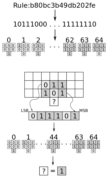
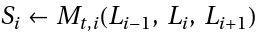Here we have introduced the array S which is an intermediate ledge. What we have here is that at step t the new symbol in the intermediate ledge(S) at position i  will be given by the operator located in the maze(M) at step t and position i. Said operator only takes the three symbols in L located at positions i – 1,i  , i + 1.

The Operator Alphabet

Given what we know above we can no start to look at the specific operators. We will use a somewhat different notation where:This makes the description of the operators more intuitive. Below follows a list of the different operators: 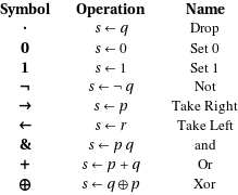These are all the operators we will use except for  the jump operator but i will implement that later.

Example: 3-Bit Ripple-Carry Adder

Well here i will show you the code for a very simple three bit ripple-carry adder which will take two 3 bit numbers, add them and produce a 4 bit output. To do this we will connect three full-adders so obviously the first step will be to construct a simple full-adder. A full adder takes the bits A,B,C and outputs two bits S and Co where S is the sum A+B+C and Co is the carry out bit. The formula for S and Co is:

To do this we will configure the Maze as follows, With the specific positions for the input and output marked:

And then we just take three of these and connect them together using a chain of Take Left and Take Right and we get a 3-Bit adder:

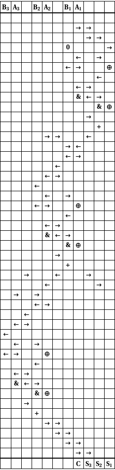And isn’t that just pretty awesome!
Now lets see if it works! I will just Configure the ledge to correspond to 7+5 which would in binary be 111(A)+101(B). We know that 7+5=12 so we would be expecting to see That the last four bits on the ground are 1100. So then let’s try it! Below i will show all of the steps in the operation:
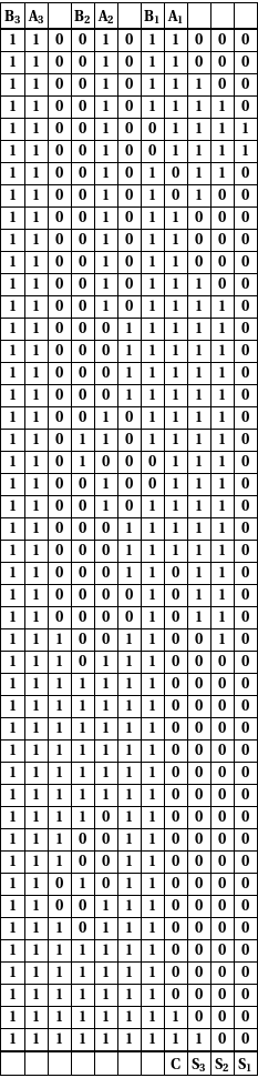And it works! How incredibly neat!!

Whats next?

Well that’s it for this brief introduction. I will soon follow-up this post with a more detailed description on its operation and the “assembler” which i have written for the system. Later  we will also implement the special jump operator(although i might have to do a complete rewrite of the code to get that working).

And one day there will be a more popper analysis the system.

I’m fully aware that i probably explained this in the most confusing and incoherent way so please don’t be afraid to ask any questions or leave feedback!

Keep it Real!
//The Grandmother